Overview
This tutorial demonstrates the basic capabilities of the AutoGP package.
import AutoGPimport CSV
import Dates
import DataFrames
using PyPlot: pltLoading Data
The first step is to load a dataset from disk. The tsdl.161.csv file, obtained from the Time Series Data Library, has two columns:
dsindicates time stamps.yindicates measured time series values.
In the call to CSV.File, we explicitly set the type of the ds column to Dates.Date, permitted types for time indexes are types T <: Real and T < :Dates.TimeType, see AutoGP.IndexType.
data = CSV.File("assets/tsdl.161.csv"; header=[:ds, :y], types=Dict(:ds=>Dates.Date, :y=>Float64));
df = DataFrames.DataFrame(data)
show(df)[1m [0m│ ds y
─────┼───────────────────
1 │ 1949-01-01 112.0
2 │ 1949-02-01 118.0
3 │ 1949-03-01 132.0
4 │ 1949-04-01 129.0
5 │ 1949-05-01 121.0
6 │ 1949-06-01 135.0
7 │ 1949-07-01 148.0
8 │ 1949-08-01 148.0
9 │ 1949-09-01 136.0
10 │ 1949-10-01 119.0
11 │ 1949-11-01 104.0
12 │ 1949-12-01 118.0
⋮ │ ⋮ ⋮
134 │ 1960-02-01 391.0
135 │ 1960-03-01 419.0
136 │ 1960-04-01 461.0
137 │ 1960-05-01 472.0
138 │ 1960-06-01 535.0
139 │ 1960-07-01 622.0
140 │ 1960-08-01 606.0
141 │ 1960-09-01 508.0
142 │ 1960-10-01 461.0
143 │ 1960-11-01 390.0
144 │ 1960-12-01 432.0
[36m 121 rows omitted[0mWe next split the data into a training set and test set.
n_test = 18
n_train = DataFrames.nrow(df) - n_test
df_train = df[1:end-n_test, :]
df_test = df[end-n_test+1:end, :]

fig, ax = plt.subplots(figsize=(10,5))
ax.scatter(df_train.ds, df_train.y, marker=".", color="k", label="Observed Data")
ax.scatter(df_test.ds, df_test.y, marker=".", color="r", label="Test Data")
ax.legend();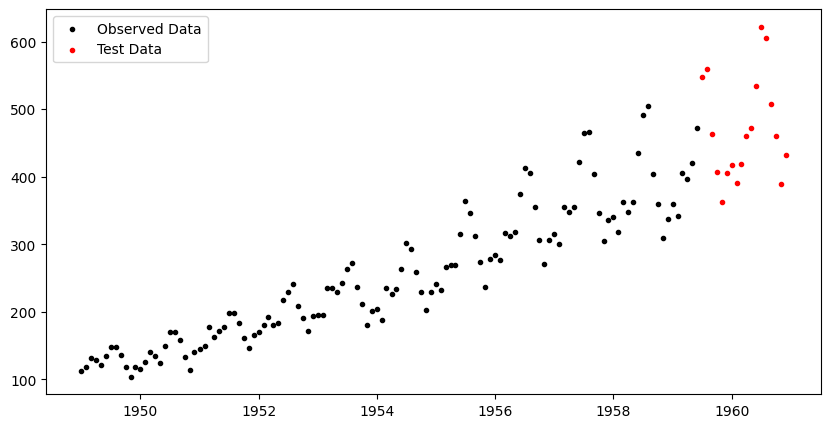
Creating an AutoGP Model
Julia natively supports multiprocessing, which greatly improves performance for embarrassingly parallel computations in AutoGP. The number of threads available to Julia can be set using the JULIA_NUM_THREADS=[nthreads] environment variable or invoking julia -t [nthreads] from the command line.
Threads.nthreads()8We next initialize a AutoGP.GPModel, which will enable us to automatically discover an ensemble of Gaussian process covariance kernels for modeling the time series data. Initially, the model structures and parameters are sampled from the prior. The n_particles argument is optional and specifices the number of particles for sequential Monte Carlo inference.
model = AutoGP.GPModel(df_train.ds, df_train.y; n_particles=6);Generating Prior Forecasts
Calling AutoGP.covariance_kernels returns the ensemble of covariance kernel structures and parameters, whose weights are given by AutoGP.particle_weights. These model structures have not yet been fitted to the data, so we are essentially importance sampling the posterior over structures and parameters given data by using the prior distribution as the proposal.
weights = AutoGP.particle_weights(model)
kernels = AutoGP.covariance_kernels(model)
for (i, (k, w)) in enumerate(zip(kernels, weights))
    println("Model $(i), Weight $(w)")
    Base.display(k)
end
Model 1, Weight 0.26142074394894477
CP(0.19055667126219877, 0.001)
├── LIN(1.26; 3.19, 0.06)
└── PER(0.11, 0.52; 0.13)
Model 2, Weight 4.0257929388061755e-27
LIN(0.09; 0.52, 0.20)
Model 3, Weight 1.7975106803349286e-9
PER(1.37, 0.30; 1.04)
Model 4, Weight 1.1645819463329054e-21
GE(0.42, 1.00; 0.04)
Model 5, Weight 7.24814391228416e-39
×
├── GE(0.09, 0.54; 1.82)
└── PER(0.18, 0.14; 0.42)
Model 6, Weight 0.7385792542535452
GE(0.13, 0.29; 0.11)Forecasts are obtained using AutoGP.predict, which takes in a model, a list of time points ds (which we specify to be the observed time points, the test time points, and 36 months of future time points). We also specify a list of quantiles for obtaining prediction intervals. The return value is a DataFrames.DataFrame object that show the particle id, particle weight, and predictions from each of the particles in model.
ds_future = range(start=df.ds[end]+Dates.Month(1), step=Dates.Month(1), length=36)
ds_query = vcat(df_train.ds, df_test.ds, ds_future)
forecasts = AutoGP.predict(model, ds_query; quantiles=[0.025, 0.975])
show(forecasts)[1m [0m│ ds particle weight y_0.025 y_0.975 y_mean
──────┼────────────────────────────────────────────────────────────
1 │ 1949-01-01 1 0.261421 -83.3461 347.688 132.171
2 │ 1949-02-01 1 0.261421 -83.1647 347.645 132.24
3 │ 1949-03-01 1 0.261421 -83.0097 347.615 132.303
4 │ 1949-04-01 1 0.261421 -82.8478 347.592 132.372
5 │ 1949-05-01 1 0.261421 -82.7009 347.579 132.439
6 │ 1949-06-01 1 0.261421 -82.5592 347.576 132.508
7 │ 1949-07-01 1 0.261421 -82.4319 347.583 132.575
8 │ 1949-08-01 1 0.261421 -82.3105 347.6 132.645
9 │ 1949-09-01 1 0.261421 -82.1993 347.627 132.714
10 │ 1949-10-01 1 0.261421 -82.1016 347.664 132.781
11 │ 1949-11-01 1 0.261421 -82.0108 347.711 132.85
12 │ 1949-12-01 1 0.261421 -81.9328 347.767 132.917
⋮ │ ⋮ ⋮ ⋮ ⋮ ⋮ ⋮
1070 │ 1963-02-01 6 0.738579 -71.2452 656.635 292.695
1071 │ 1963-03-01 6 0.738579 -71.8672 656.291 292.212
1072 │ 1963-04-01 6 0.738579 -72.5386 655.92 291.691
1073 │ 1963-05-01 6 0.738579 -73.1719 655.57 291.199
1074 │ 1963-06-01 6 0.738579 -73.8099 655.217 290.703
1075 │ 1963-07-01 6 0.738579 -74.4122 654.883 290.235
1076 │ 1963-08-01 6 0.738579 -75.0194 654.546 289.763
1077 │ 1963-09-01 6 0.738579 -75.6119 654.218 289.303
1078 │ 1963-10-01 6 0.738579 -76.1718 653.907 288.868
1079 │ 1963-11-01 6 0.738579 -76.7368 653.594 288.428
1080 │ 1963-12-01 6 0.738579 -77.2711 653.297 288.013
[36m 1057 rows omitted[0mLet us visualize the forecasts before model fitting. The model clearly underfits the data.
fig, ax = plt.subplots(figsize=(10,5))

ax.scatter(df_train.ds, df_train.y, marker=".", color="k", label="Observed Data")
ax.scatter(df_test.ds, df_test.y, marker=".", color="r", label="Test Data")

for i=1:AutoGP.num_particles(model)
    subdf = forecasts[forecasts.particle.==i,:]
    ax.plot(subdf[!,"ds"], subdf[!,"y_mean"], color="k", linewidth=.5)
    ax.fill_between(
        subdf.ds, subdf[!,"y_0.025"], subdf[!,"y_0.975"];
        color="tab:blue", alpha=0.05)
end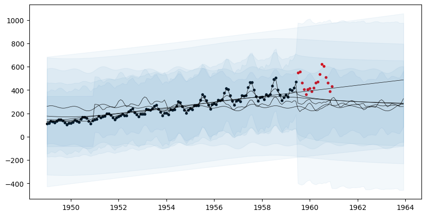
Model Fitting via SMC
The next step is to fit the model to the observed data. There are three fitting algorithms available. We will use AutoGP.fit_smc! which leverages sequential Monte Carlo structure learning to infer the covariance kernel structures and parameters.
The annealing schedule below adds roughly 10% of the observed data at each step, with 100 MCMC rejuvenation steps over the structure and 10 Hamiltonian Monte Carlo steps for the parameters. Using verbose=true will print some statistics about the acceptance rates of difference MCMC and HMC moves that are performed within the SMC learning algorithm.
AutoGP.seed!(6)
AutoGP.fit_smc!(model; schedule=AutoGP.Schedule.linear_schedule(n_train, .10), n_mcmc=75, n_hmc=10, verbose=true);
Running SMC round 13/126
weights [2.14e-01, 5.85e-02, 2.05e-01, 5.23e-01, 1.09e-04, 1.51e-04]
resampled true
accepted MCMC[12/75] HMC[71/78]
accepted MCMC[9/75] HMC[64/69]
accepted MCMC[19/75] HMC[122/132]
accepted MCMC[22/75] HMC[121/136]
accepted MCMC[22/75] HMC[89/107]
accepted MCMC[27/75] HMC[191/202]
Running SMC round 26/126
weights [8.08e-03, 4.24e-01, 1.10e-03, 1.92e-02, 3.97e-01, 1.50e-01]
resampled true
accepted MCMC[7/75] HMC[55/58]
accepted MCMC[6/75] HMC[37/40]
accepted MCMC[6/75] HMC[43/47]
accepted MCMC[12/75] HMC[52/60]
accepted MCMC[18/75] HMC[84/97]
accepted MCMC[21/75] HMC[112/125]
Running SMC round 39/126
weights [1.99e-02, 1.74e-01, 3.01e-02, 4.08e-02, 1.95e-02, 7.16e-01]
resampled true
accepted MCMC[0/75] HMC[0/0]
accepted MCMC[1/75] HMC[6/7]
accepted MCMC[5/75] HMC[43/44]
accepted MCMC[13/75] HMC[50/61]
accepted MCMC[10/75] HMC[64/71]
accepted MCMC[17/75] HMC[95/105]
Running SMC round 52/126
weights [1.66e-03, 8.13e-02, 8.69e-02, 1.65e-01, 4.54e-02, 6.20e-01]
resampled true
accepted MCMC[3/75] HMC[24/25]
accepted MCMC[4/75] HMC[24/27]
accepted MCMC[11/75] HMC[25/36]
accepted MCMC[17/75] HMC[111/122]
accepted MCMC[23/75] HMC[62/84]
accepted MCMC[24/75] HMC[92/114]
Running SMC round 65/126
weights [3.87e-02, 5.07e-01, 7.59e-03, 1.50e-01, 5.29e-02, 2.44e-01]
resampled true
accepted MCMC[0/75] HMC[0/0]
accepted MCMC[18/75] HMC[7/25]
accepted MCMC[20/75] HMC[11/31]
accepted MCMC[28/75] HMC[27/55]
accepted MCMC[26/75] HMC[25/51]
accepted MCMC[27/75] HMC[35/62]
Running SMC round 78/126
weights [5.42e-06, 2.46e-04, 1.94e-04, 3.56e-04, 9.42e-01, 5.75e-02]
resampled true
accepted MCMC[14/75] HMC[0/14]
accepted MCMC[14/75] HMC[0/14]
accepted MCMC[17/75] HMC[0/17]
accepted MCMC[15/75] HMC[2/17]
accepted MCMC[26/75] HMC[2/28]
accepted MCMC[18/75] HMC[0/18]
Running SMC round 91/126
weights [5.03e-02, 1.90e-04, 3.17e-01, 9.72e-02, 1.74e-01, 3.61e-01]
resampled false
accepted MCMC[16/75] HMC[0/16]
accepted MCMC[15/75] HMC[0/15]
accepted MCMC[12/75] HMC[0/12]
accepted MCMC[16/75] HMC[0/16]
accepted MCMC[18/75] HMC[0/18]
accepted MCMC[28/75] HMC[1/29]
Running SMC round 104/126
weights [1.14e-02, 6.30e-08, 7.42e-02, 6.76e-01, 1.48e-01, 9.09e-02]
resampled true
accepted MCMC[15/75] HMC[0/15]
accepted MCMC[14/75] HMC[0/14]
accepted MCMC[12/75] HMC[0/12]
accepted MCMC[16/75] HMC[0/16]
accepted MCMC[15/75] HMC[1/16]
accepted MCMC[30/75] HMC[0/30]
Running SMC round 117/126
weights [3.84e-01, 4.30e-02, 2.19e-01, 1.02e-01, 1.59e-01, 9.31e-02]
resampled false
accepted MCMC[9/75] HMC[0/9]
accepted MCMC[15/75] HMC[0/15]
accepted MCMC[20/75] HMC[1/21]
accepted MCMC[15/75] HMC[0/15]
accepted MCMC[17/75] HMC[0/17]
accepted MCMC[20/75] HMC[0/20]
Running SMC round 126/126
weights [5.19e-01, 3.88e-02, 5.85e-02, 1.22e-01, 9.97e-02, 1.62e-01]
accepted MCMC[10/75] HMC[0/10]
accepted MCMC[15/75] HMC[0/15]
accepted MCMC[13/75] HMC[1/14]
accepted MCMC[20/75] HMC[0/20]
accepted MCMC[17/75] HMC[0/17]
accepted MCMC[24/75] HMC[0/24]Generating Posterior Forecasts
Having the fit data, we can now inspect the ensemble of posterior structures, parameters, and predictions.
ds_future = range(start=df_test.ds[end]+Dates.Month(1), step=Dates.Month(1), length=36)
ds_query = vcat(df_train.ds, df_test.ds, ds_future)
forecasts = AutoGP.predict(model, ds_query; quantiles=[0.025, 0.975]);
show(forecasts)[1m [0m│ ds particle weight y_0.025 y_0.975 y_mean
──────┼─────────────────────────────────────────────────────────────
1 │ 1949-01-01 1 0.518786 95.7778 124.096 109.937
2 │ 1949-02-01 1 0.518786 105.533 132.895 119.214
3 │ 1949-03-01 1 0.518786 118.461 145.764 132.113
4 │ 1949-04-01 1 0.518786 112.317 139.654 125.985
5 │ 1949-05-01 1 0.518786 106.34 133.628 119.984
6 │ 1949-06-01 1 0.518786 118.932 146.186 132.559
7 │ 1949-07-01 1 0.518786 131.405 158.626 145.016
8 │ 1949-08-01 1 0.518786 132.641 159.89 146.266
9 │ 1949-09-01 1 0.518786 122.15 149.355 135.753
10 │ 1949-10-01 1 0.518786 104.155 131.338 117.746
11 │ 1949-11-01 1 0.518786 92.5327 119.705 106.119
12 │ 1949-12-01 1 0.518786 102.479 129.31 115.894
⋮ │ ⋮ ⋮ ⋮ ⋮ ⋮ ⋮
1070 │ 1963-02-01 6 0.162471 264.78 700.582 482.681
1071 │ 1963-03-01 6 0.162471 334.241 779.225 556.733
1072 │ 1963-04-01 6 0.162471 318.448 773.472 545.96
1073 │ 1963-05-01 6 0.162471 345.825 809.683 577.754
1074 │ 1963-06-01 6 0.162471 449.011 921.948 685.479
1075 │ 1963-07-01 6 0.162471 556.444 1049.52 802.984
1076 │ 1963-08-01 6 0.162471 576.012 1085.92 830.965
1077 │ 1963-09-01 6 0.162471 408.099 932.331 670.215
1078 │ 1963-10-01 6 0.162471 299.235 837.312 568.274
1079 │ 1963-11-01 6 0.162471 216.275 768.47 492.373
1080 │ 1963-12-01 6 0.162471 240.204 805.597 522.9
[36m 1057 rows omitted[0mThe plot below reflects posterior uncertainty as to whether the linear componenet will persist or the data will revert to the mean.
fig, ax = plt.subplots(figsize=(10,5))
ax.scatter(df_train.ds, df_train.y, marker=".", color="k", label="Observed Data")
ax.scatter(df_test.ds, df_test.y, marker=".", color="r", label="Test Data")

for i=1:AutoGP.num_particles(model)
    subdf = forecasts[forecasts.particle.==i,:]
    ax.plot(subdf[!,"ds"], subdf[!,"y_mean"], color="k", linewidth=.5)
    ax.fill_between(
        subdf.ds, subdf[!,"y_0.025"], subdf[!,"y_0.975"];
        color="tab:blue", alpha=0.05)
end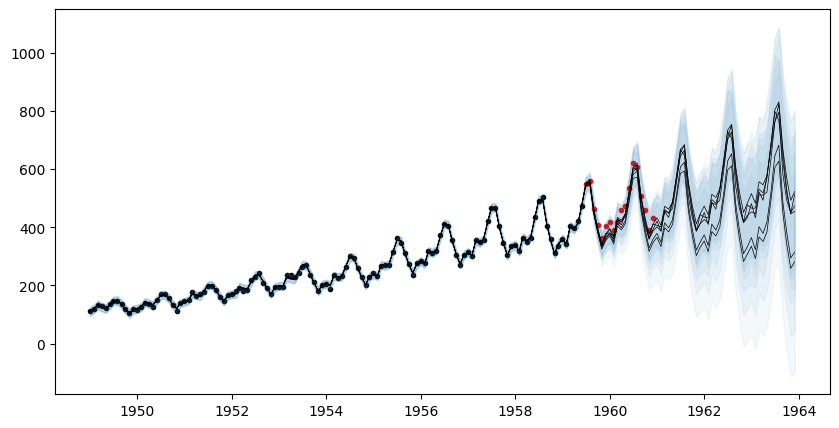
We can also inspect the discovered kernel structures and their weights.
weights = AutoGP.particle_weights(model)
kernels = AutoGP.covariance_kernels(model)
for (i, (k, w)) in enumerate(zip(kernels, weights))
    println("Model $(i), Weight $(w)")
    display(k)
end
Model 1, Weight 0.5187856913664618
+
├── ×
│ ├── LIN(0.58; 0.56, 0.19)
│ └── +
│ ├── LIN(0.19; 0.92, 0.79)
│ └── ×
│ ├── LIN(0.05; 0.02, 0.38)
│ └── +
│ ├── PER(0.78, 0.10; 0.20)
│ └── GE(0.72, 1.43; 0.11)
└── ×
├── LIN(0.16; 0.55, 0.51)
└── ×
├── LIN(0.06; 0.16, 0.08)
└── LIN(0.22; 0.07, 0.46)
Model 2, Weight 0.0388018393363426
×
├── LIN(0.38; 0.08, 0.92)
└── +
├── ×
│ ├── LIN(0.58; 0.13, 0.07)
│ └── GE(0.56, 1.51; 0.69)
└── ×
├── LIN(0.05; 0.10, 0.70)
└── PER(0.48, 0.10; 0.17)
Model 3, Weight 0.05854237186951741
×
├── LIN(0.06; 0.12, 0.55)
└── +
├── LIN(0.06; 0.83, 0.20)
└── ×
├── LIN(0.05; 0.03, 0.37)
└── +
├── PER(0.35, 0.10; 0.13)
└── GE(0.58, 1.50; 0.20)
Model 4, Weight 0.12171996350432317
×
├── LIN(0.07; 0.12, 0.50)
└── +
├── ×
│ ├── LIN(0.07; 0.08, 0.19)
│ └── GE(0.56, 1.51; 0.69)
└── ×
├── LIN(0.30; 0.13, 0.27)
└── PER(0.48, 0.10; 0.17)
Model 5, Weight 0.09967934632668538
×
├── LIN(0.33; 0.08, 0.84)
└── +
├── ×
│ ├── LIN(0.40; 0.13, 0.07)
│ └── GE(0.69, 1.28; 0.33)
└── ×
├── LIN(0.26; 0.10, 0.30)
└── +
├── PER(0.54, 0.10; 0.14)
└── LIN(0.52; 0.59, 0.21)
Model 6, Weight 0.16247078759667166
×
├── LIN(0.31; 0.12, 0.32)
└── +
├── ×
│ ├── LIN(0.22; 0.21, 0.23)
│ └── +
│ ├── ×
│ │ ├── LIN(0.30; 0.24, 0.92)
│ │ └── LIN(0.10; 1.53, 0.25)
│ └── +
│ ├── GE(0.23, 1.25; 0.06)
│ └── LIN(0.04; 0.34, 0.08)
└── ×
├── LIN(0.38; 0.28, 0.27)
└── PER(0.48, 0.10; 0.17)Computing Predictive Probabilities
In addition to generating forecasts, the predictive probability of new data can be computed by using AutoGP.predict_proba. The table below shows that the particles in our collection are able to predict the future data with varying accuracy, illustrating the benefits of maintaining an ensemble of learned structures.
logps = AutoGP.predict_proba(model, df_test.ds, df_test.y);
show(logps)[1m [0m│ particle weight logp
───┼───────────────────────────────
1 │ 1 0.518786 -81.0226
2 │ 2 0.0388018 -80.4687
3 │ 3 0.0585424 -78.3537
4 │ 4 0.12172 -79.2853
5 │ 5 0.0996793 -79.5163
6 │ 6 0.162471 -77.2665It is also possible to directly access the underlying predictive distribution of new data at arbitrary time series values by using AutoGP.predict_mvn, which returns an instance of Distributions.MixtureModel. The Distributions.MvNormal object corresponding to each of the 7 particles in the mixture can be extracted using Distributions.components and the weights extracted using Distributions.probs.
Each MvNormal in the mixture has 18 dimensions corresponding to the length of df_test.ds.
mvn = AutoGP.predict_mvn(model, df_test.ds)MixtureModel{Distributions.MvNormal}(K = 6)
components[1] (prior = 0.5188): FullNormal(
dim: 18
μ: [550.0466055631144, 543.5685832436789, 458.0672732626237, 387.83042059450264, 336.3274841090669, 378.84360283044555, 380.7405954069613, 370.5597600287218, 428.60605677444596, 417.8272939610252, 445.710229207111, 527.722968622132, 606.5232420193234, 592.7113473338969, 495.58143177869687, 415.9744653512393, 361.6811541092175, 410.86491959299735]
Σ: [110.43133996791498 70.43337927366102 … 106.0193369583544 105.68013071952048; 70.43337927366102 157.2315611083291 … 175.7899821967875 176.06414206239037; … ; 106.0193369583544 175.7899821967875 … 1289.6029024068575 1266.7465844069018; 105.68013071952048 176.06414206239037 … 1266.7465844069018 1402.6718895178888]
)
components[2] (prior = 0.0388): FullNormal(
dim: 18
μ: [550.0896881260433, 557.9183559988504, 451.7397701335289, 387.6936971300408, 330.34991142470057, 359.2956794851918, 378.39571104805384, 350.04141045569975, 413.64406521435524, 398.5566703647475, 422.68213778752005, 500.29404572255766, 582.8353873538858, 592.0046117753294, 465.11743221070196, 393.04897063058206, 329.267681609935, 358.99798544788507]
Σ: [170.0085073382823 105.25012857653914 … 177.47794790860507 175.32855445033792; 105.25012857653914 238.13684073916644 … 293.4524054906246 290.979138749098; … ; 177.47794790860507 293.4524054906246 … 2416.364949433486 2381.6802393098687; 175.32855445033792 290.979138749098 … 2381.6802393098687 2639.691137455322]
)
components[3] (prior = 0.0585): FullNormal(
dim: 18
μ: [544.0602736685337, 552.3149196264309, 443.2068512785211, 383.4411432273028, 333.1461848874234, 363.8639799436975, 380.29770568852405, 358.75477706207874, 423.7049992204387, 408.1716555603478, 445.55695338552516, 518.8219447058625, 591.4986944066081, 605.5457079908405, 470.62796484325577, 405.9325078335371, 358.7557037493446, 386.64043978162846]
Σ: [169.219485798796 95.5607024083134 … 186.32839433051615 187.43906631934843; 95.5607024083134 226.17368143388276 … 296.7553075541498 297.9986486627047; … ; 186.32839433051615 296.7553075541498 … 2674.2672217311588 2576.455195366638; 187.43906631934843 297.9986486627047 … 2576.455195366638 2939.5711056844825]
)
components[4] (prior = 0.1217): FullNormal(
dim: 18
μ: [543.6216230023799, 547.0922547835243, 446.04078249000014, 380.61770131619136, 324.29212851917504, 353.77691026184584, 371.1395407479827, 342.34364108088573, 404.0153377656334, 390.97432104186356, 413.05844950054205, 491.9302348550482, 568.3911582492668, 571.8976295358883, 452.94290011076225, 379.16919720465506, 317.0536108758739, 347.69198390460025]
Σ: [190.70740795818799 154.7146370830134 … 264.57139974473904 263.6724500005631; 154.7146370830134 321.7637732335915 … 489.4185844326134 488.7990902096624; … ; 264.57139974473904 489.4185844326134 … 4640.723077886049 4724.747558194855; 263.6724500005631 488.7990902096624 … 4724.747558194855 5100.627801272796]
)
components[5] (prior = 0.0997): FullNormal(
dim: 18
μ: [552.7093727527794, 563.9629154045222, 463.17633751362314, 397.0289509923992, 340.6980456518664, 369.3109007416625, 393.9776845927133, 364.4534810210352, 428.49669476215763, 419.62843208711365, 437.11650012898417, 518.4548245910088, 604.432782069657, 621.3790060721707, 502.57788998868597, 426.35148491965776, 363.78741844671123, 392.4909178791416]
Σ: [163.93677598232696 101.84796443535812 … 150.19871047085653 148.021181862565; 101.84796443535812 230.96594095228826 … 248.28364894831142 246.73036788677837; … ; 150.19871047085653 248.28364894831142 … 1894.8528328890138 1837.9190390714505; 148.021181862565 246.73036788677837 … 1837.9190390714505 2060.0738352212666]
)
components[6] (prior = 0.1625): FullNormal(
dim: 18
μ: [547.7766511058762, 554.0371551300294, 458.7231316164908, 395.94898562441665, 343.42395227426294, 375.81336956905994, 396.18401584832765, 371.80967668657166, 434.12203157338473, 424.18770474918983, 446.63575317375114, 526.406634220377, 606.4956206078521, 613.7056476449546, 502.8621955266556, 432.7728333122789, 375.92004227567435, 410.64183137650747]
Σ: [155.68263652531186 105.08831951166466 … 153.16479636831943 151.89660431693395; 105.08831951166466 230.1409831228302 … 262.3355496966857 260.5635431735595; … ; 153.16479636831943 262.3355496966857 … 2040.7723016580135 2008.230949860343; 151.89660431693395 260.5635431735595 … 2008.230949860343 2220.8419553962394]
)Operations from the Distributions package can now be applied to the mvn object.
Incorporating New Data
Online learning is supported by using AutoGP.add_data!, which lets us incorporate a new batch of observations. Each particle's weight will be updated based on how well it predicts the new data (technically, the predictive probability it assigns to the new observations). Before adding new data, let us first look at the current particle weights.
AutoGP.particle_weights(model)6-element Vector{Float64}:
0.5187856913664618
0.0388018393363426
0.05854237186951741
0.12171996350432317
0.09967934632668538
0.16247078759667166Here are the forecasts and predictive probabilities of the test data under each particle in model.
using Printf: @sprintfforecasts = AutoGP.predict(model, df_test.ds; quantiles=[0.025, 0.975])
fig, axes = plt.subplots(ncols=6)
for i=1:AutoGP.num_particles(model)
axes[i].scatter(df_test.ds, df_test.y, marker=".", color="r", label="Test Data")
subdf = forecasts[forecasts.particle.==i,:]
axes[i].plot(subdf[!,"ds"], subdf[!,"y_mean"], color="k", linewidth=.5)
axes[i].fill_between(
subdf.ds, subdf[!,"y_0.025"], subdf[!,"y_0.975"];
color="tab:blue", alpha=0.1)
axes[i].set_title("$(i), logp $(@sprintf "%1.2f" logps[i,:logp])")
axes[i].set_yticks([])
axes[i].set_ylim([0.8*minimum(df_test.y), 1.1*maximum(df_test.y)])
axes[i].tick_params(axis="x", labelrotation=90)
fig.set_size_inches(12, 5)
fig.set_tight_layout(true)
end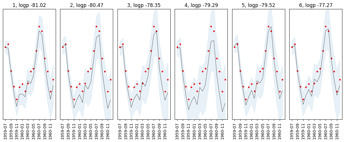
Now let's incorporate the data and see what happens to the particle weights.
AutoGP.add_data!(model, df_test.ds, df_test.y)
AutoGP.particle_weights(model)
6-element Vector{Float64}:
0.054480109584894444
0.007089917054484329
0.08867768509766472
0.07262818579191704
0.04720986321304457
0.7299142392579898The particle weights have changed to reflect the fact that some particles are able to predict the new data better than others, which indicates they are able to better capture the underlying data generating process. The particles can be resampled using AutoGP.maybe_resample!, we will use an effective sample size of num_particles(model)/2 as the resampling criterion.
AutoGP.maybe_resample!(model, AutoGP.num_particles(model)/2)trueBecause the resampling critereon was met, the particles were resampled and now have equal weights.
AutoGP.particle_weights(model)6-element Vector{Float64}:
0.16666666666666669
0.16666666666666669
0.16666666666666669
0.16666666666666669
0.16666666666666669
0.16666666666666669The estimate of the marginal likelihood can be computed using AutoGP.log_marginal_likelihood_estimate.
AutoGP.log_marginal_likelihood_estimate(model)214.57030788045827Since we have added new data, we can update the particle structures and parameters by using AutoGP.mcmc_structure!. Note that this "particle rejuvenation" operation does not impact the weights.
AutoGP.mcmc_structure!(model, 100, 10; verbose=true)accepted MCMC[19/100] HMC[0/38]
accepted MCMC[27/100] HMC[0/54]
accepted MCMC[23/100] HMC[0/46]
accepted MCMC[25/100] HMC[0/50]
accepted MCMC[26/100] HMC[0/52]
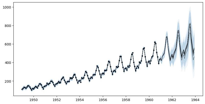
accepted MCMC[25/100] HMC[0/50]Let's generate and plot the forecasts over the 36 month period again now that we have observed all the data. The prediction intervals are markedly narrower and it is more likely that the linear trend will persist rather than revert.
forecasts = AutoGP.predict(model, ds_query; quantiles=[0.025, 0.975]);

fig, ax = plt.subplots(figsize=(10,5))
ax.scatter(df.ds, df.y, marker=".", color="k", label="Observed Data")
for i=1:AutoGP.num_particles(model)
    subdf = forecasts[forecasts.particle.==i,:]
    ax.plot(subdf[!,"ds"], subdf[!,"y_mean"], color="k", linewidth=.5)
    ax.fill_between(
        subdf.ds, subdf[!,"y_0.025"], subdf[!,"y_0.975"];
        color="tab:blue", alpha=0.05)
end