Greedy Search and MCMC

The Model Fitting via SMC section of the Overview tutorial showed how to learn the structure of Gaussian process time series models by using sequential Monte Carlo structure learning. This tutorial will illustrate two alternative structure discovery methods:

1. Greedy search (AutoGP.fit_greedy!)
2. MCMC sampling (AutoGP.fit_mcmc!)

import AutoGP
import CSV
import Dates
import DataFrames
import Distributions

using AutoGP.GP
using PyPlot: plt

The synthetic data generated below is the same as the data used in the Inspecting Online Inference tutorial.

AutoGP.seed!(2)
cov = (Linear(1,0,50) * Periodic(5,2)) + GammaExponential(1,1)
noise = .1
n = 100

ds = Vector{Float64}(range(0, 20, length=n))
dist = Distributions.MvNormal(cov, noise, Float64[], Float64[], ds)
y = Distributions.rand(dist);

fig, ax = plt.subplots(figsize=(6, 4), dpi=100, tight_layout=true)
ax.plot(ds, y, marker=".", markerfacecolor="none", markeredgecolor="k", color="black");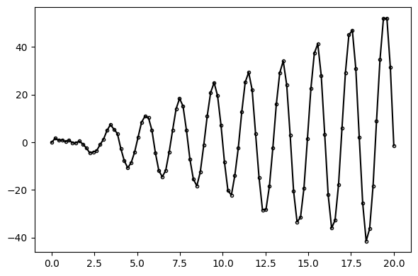

Greedy Search

To perform greedy search, the model::GPModel object must have a single particle. Moreover, greedy search does not currently supported AutoGP.GP.ChangePoint covariance structures. We can disable changepoints by using a custom AutoGP.GP.GPConfig, as shown below.

model = AutoGP.GPModel(ds, y; n_particles=1, config=GP.GPConfig(changepoints=false));

Greedy search also supports callback functions to inspect inference. The callback function below will be invoked at each stage of the greedy search. We will plot AIC at each stage and the corresponding covariance structure.

fig, axs = plt.subplots(nrows=2, ncols=5, figsize=(15, 15), dpi=150)
axs = permutedims(axs)
fig.set_tight_layout(true)
plt.close(fig)

function fn_callback(; kwargs...)
    model = kwargs[:model]
    step = kwargs[:step]
    aic = kwargs[:aic]
    
    ds_query = vcat(model.ds, (20:.1:30))
    predictions = AutoGP.predict(model, ds_query; quantiles=[0.025, 0.975])
    
    axs[step].scatter(model.ds, model.y, marker="o", color="k", s=10, label="Observed Data")    
    axs[step].axvline(model.ds[end], color="red", linestyle="--")
    axs[step].plot(predictions[!,:ds], predictions[!,:y_mean], linewidth=1, color="k")
    axs[step].fill_between(
        predictions[!,:ds],
        predictions[!,"y_0.025"],
        predictions[!,"y_0.975"],
        color="tab:green",
        alpha=.25)

    io = IOBuffer()
    cov = AutoGP.covariance_kernels(model)[1]
    Base.show(io, MIME("text/plain"), cov)
    cov_str = String(take!(io))
    axs[step].set_title("Step $(step)\nAIC:$(aic)\n$(cov_str)", ha="left")
end

fn_callback (generic function with 1 method)

The plots below show a key shortcoming of greedy search. Whereas steps 3–8 contain a sensible covariance structure, at steps 9–10 the structure becomes worse. This behavior is a result of greedy search selecting covariance structures with the smallest AIC, which is a rough heuristic to an ideal scoring function based on the marginal likelihood of the data under each structure, integrating out the parameter. Since AIC is based on maximum likelihood estimation and the likelihood of parameters is highly multimodal for structures such as AutoGP.GP.Periodic, greedy search may result in brittle and unpredictable behavior.

AutoGP.fit_greedy!(model; max_depth=10, callback_fn=fn_callback);
fig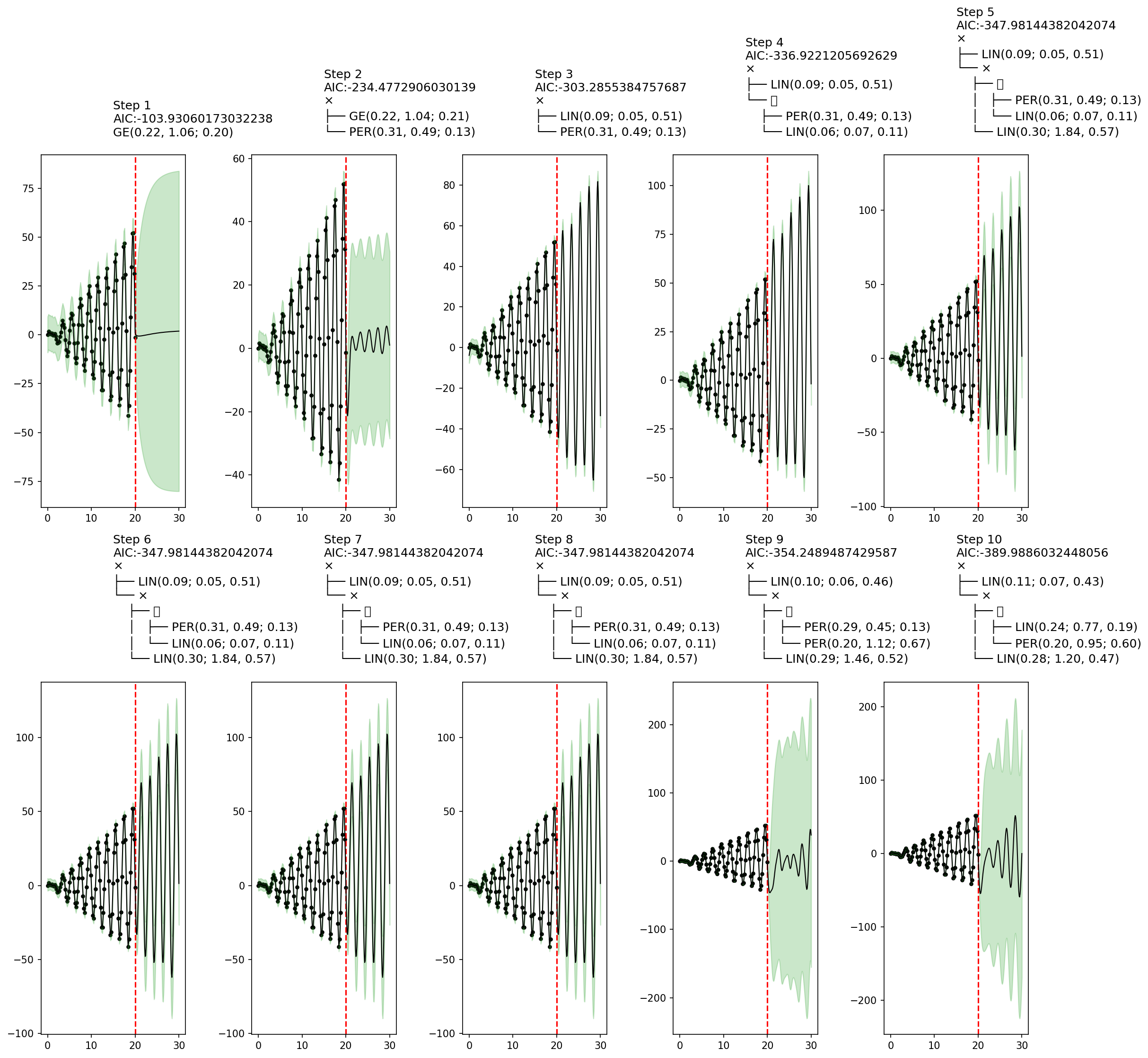

sys:1: UserWarning: Glyph 65291 (\N{FULLWIDTH PLUS SIGN}) missing from current font.

MCMC

Markov chain Monte Carlo sampling is another structure learning method. Let us initialize a GPModel with 2 particles.

model = AutoGP.GPModel(ds, y; n_particles=2);

figures = []
function fn_callback(; kwargs...)
    model = kwargs[:model]
    step = kwargs[:step]
    elapsed = kwargs[:elapsed]

    ds_query = vcat(model.ds, (20:.1:100))
    predictions = AutoGP.predict(model, ds_query; quantiles=[0.025, 0.975])
    
    fig, axis = plt.subplots(ncols=2, figsize=(18, 6), dpi=200)
    for (i, ax) in enumerate(axis)
        subdf = predictions[predictions.particle.==i,:]
        ax.scatter(model.ds, model.y, marker="o", color="k", s=10, label="Observed Data")    
        ax.axvline(model.ds[end], color="red", linestyle="--")
        ax.plot(subdf[!,:ds], subdf[!,:y_mean], linewidth=1, color="k")
        ax.fill_between(
            subdf[!,:ds],
            subdf[!,"y_0.025"],
            subdf[!,"y_0.975"],
            color="tab:green",
            alpha=.25)

        io = IOBuffer()
        cov = AutoGP.covariance_kernels(model)[i]
        Base.show(io, MIME("text/plain"), cov)
        cov_str = String(take!(io))
        ax.set_title("Step $(step)\nElapsed $(elapsed[i])\n$(cov_str)", ha="left")
    end
    push!(figures, fig)
    plt.close(fig)
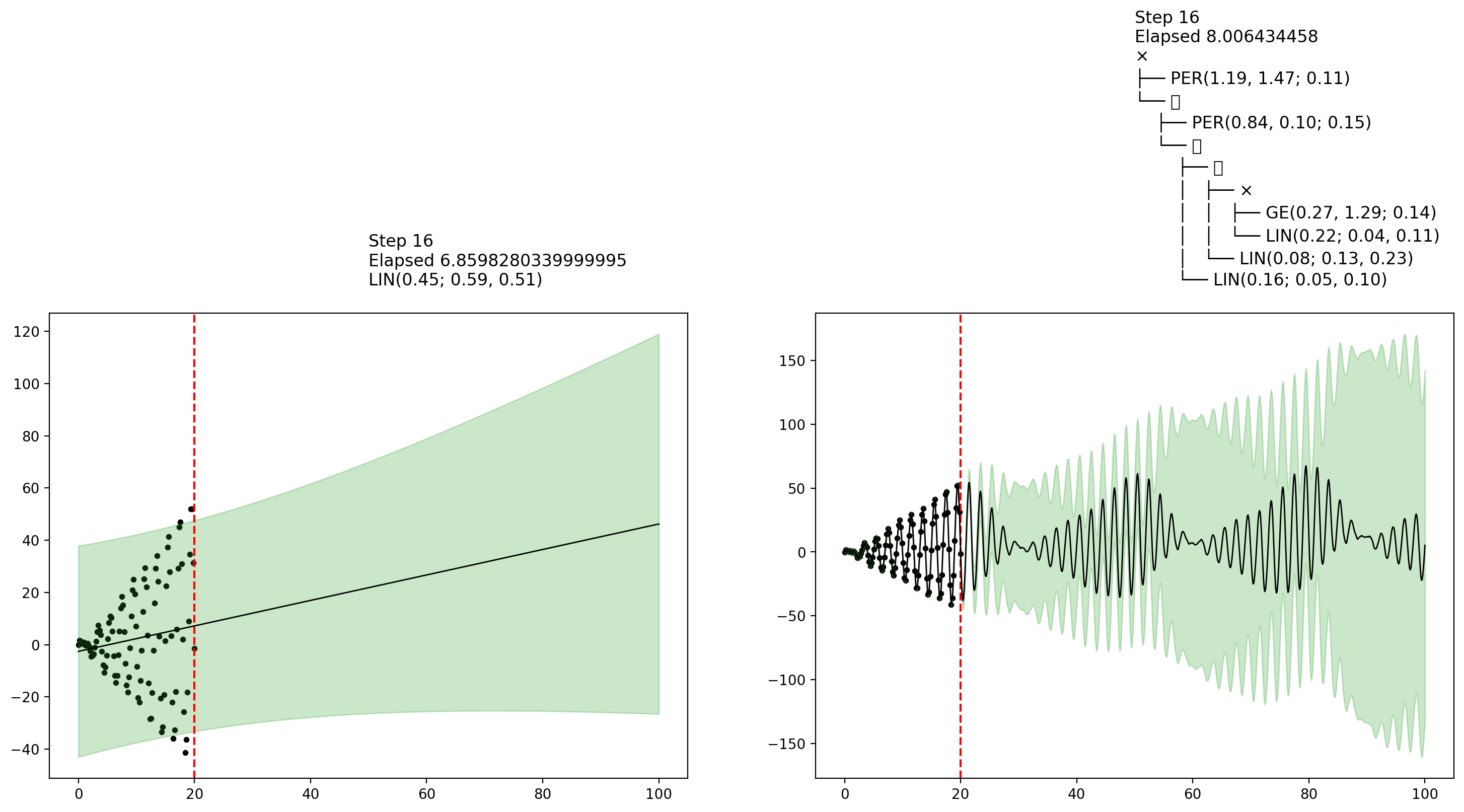
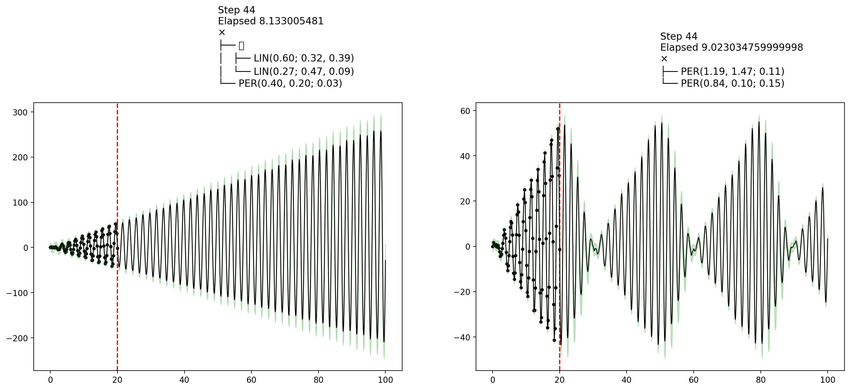
end

fn_callback (generic function with 1 method)

AutoGP.fit_mcmc!(model; n_mcmc=45, n_hmc=10, callback_fn=fn_callback)

Let's now show some plots that were collected by the callback during MCMC inference. The final plot shows an interesting example of how MCMC learning can reflect posterior uncertainty over the covariance structure.

display(figures[1])
display(figures[10])
display(figures[end])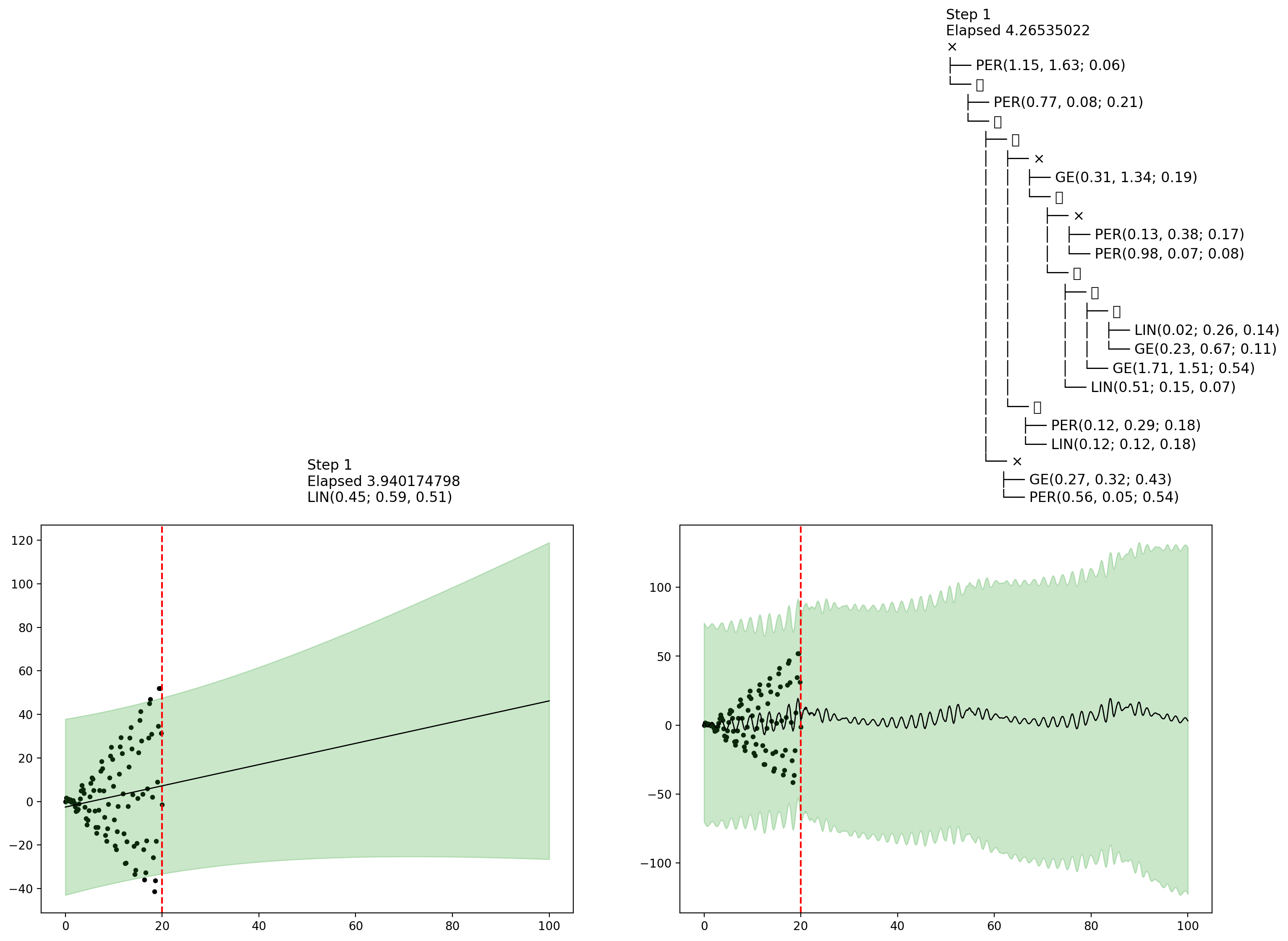

MCMC vs SMC

MCMC sampling using AutoGP.fit_mcmc! invokes the same transition kernels over structure and parameters as those used in particle rejuvenation step of AutoGP.fit_smc!. The main difference is that AutoGP.fit_smc! anneals the posterior over subsets of data at each step, whereas AutoGP.fit_mcmc! uses the full data at each step.

The benefits of SMC include

1. Runtime efficiency in cases where the structure can be quickly inferred using a subset of the data; whereas MCMC always conditions on the full data at each step yielding more expensive likelihood evaluations.
2. Principled online inference, by using AutoGP.add_data!; whereas MCMC is an offline method.
3. Particle resampling, by using AutoGP.maybe_resample!, to redirect computational effort to more promising structures and parameters; whereas MCMC iterates independent particles (i.e., chains).
4. The availability of unbiased marginal likelihood estimates (via AutoGP.log_marginal_likelihood_estimate; whereas the marginal likelihood estimate obtained from MCMC is essentially importance sampling the posterior using the prior as a proposal.